Figure 5
NOTE: Run all the code included on the “Base Code” page prior to running the following.
Setting Up
Load eigenworms and worm data of choice.
# working directory
setwd("")  # enter appropriate working directory

# load eigenworms [Broekmans et al. 2016]
ew = read.csv("eigenworms.csv", header=F, sep=",")

# load coefficients from worm of choice
data = read.csv("91 Escaping Worms/50.txt", header=F, sep="")[,1:5]
Variables
These are the optimal parameters for the data produced by Broekmans et al. 2016.
E = 5  # embedding dimension
tp = 1
theta = 2  # linearity
tau = 1

# library and prediction selection
lib = c(1,160)
pred = c(1,600)

# convert frames to seconds (i.e. indicate frames per second as fps)
fps = 20  # escaping worms
Run Functions
Run the functions created on the “Base Code” page.
# run the embedding function
matrix <- make_embed(data, E, tau, tp)

# run the prediction function
new_pred <- make_pred(E, matrix, theta, lib, pred)
observations_total = new_pred$obs
predictions_total = new_pred$pred

# run the EDM error function
errors <- edm_error(pred, observations_total, ew, predictions_total)

# run the cp error function
cp_mean <- cp_error(pred, data, ew)

# run the data classification function
new_class <- data_class(data, pred)
forward = new_class$forw
backward = new_class$back
turns = new_class$turn
change = new_class$chan
Error Plot
Create an RMS error vs time plot with colored classifications.
# setup the RMS error vs time plot
par(mai=c(0.9,0.9,0.5,0.5))
plot(c(1:length(errors))/fps, errors, col="white", xlab="time (s)", ylab="prediction error (rad)",
     cex.lab=1.5, cex.axis=1.5, xaxs="i", yaxs="i", ylim=c(0, 0.08))

# add colored rectangles for forwards, backwards, and turns
for (i in 1:length(forward)){
  rect(c(1:length(errors))[forward[i]]/fps, 0, c(1:length(errors))[forward[i]+2]/fps, 0.08,
       col="skyblue", border=NA)
}
for (i in 1:length(backward)){
  rect(c(1:length(errors))[backward[i]]/fps, 0, c(1:length(errors))[backward[i]+2]/fps, 0.08,
       col="yellow2", border=NA)
}
for (i in 1:length(turns)){
  rect(c(1:length(errors))[turns[i]]/fps, 0, c(1:length(errors))[turns[i]+2]/fps, 0.08,
       col="salmon", border=NA)
}

# add the error line on top
lines(c(1:length(errors))/fps, errors, lwd=3)
abline(h=cp_mean, lty="dashed")  # average cp error
box(col="black")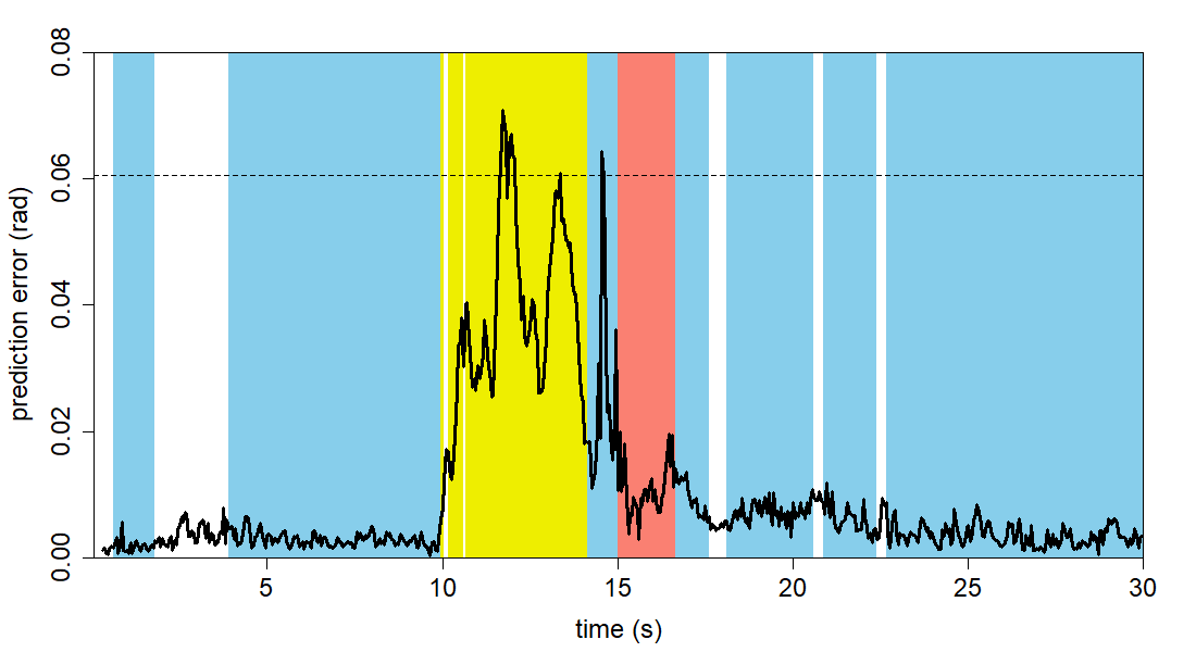
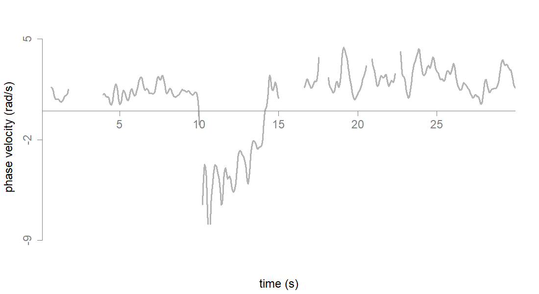
Phase Velocity Plot
Create phase velocity vs time plot with gaps at turns and unclassified sections.
# plot the phase velocity in radians per second
par(mai=c(0.9,0.9,0.5,0.5))
plot(c(2:(length(errors)-1))/fps, -10*change, type="l", xlab="time (s)",
     ylab="phase velocity (rad/s)", lwd=3, col="grey70", cex.lab=1.5, cex.axis=1.5,
     xaxs="i", yaxs="i", axes=F, ylim=c(-9.78,6.08))
abline(h=0, col="grey50")
axis(1, col="grey50", cex.lab=1.5, cex.axis=1.5, col.axis="grey50", pos=0)
axis(2, col="grey50", cex.lab=1.5, cex.axis=1.5, col.axis="grey50", at=c(-9,-2,5))